| Unnamed: 0 | patents | region | age | iscustomer |
|---|---|---|---|---|
| Loading... (need help?) |
Poisson Regression Examples
Blueprinty Case Study
Introduction
Blueprinty is a small firm that makes software for developing blueprints specifically for submitting patent applications to the US patent office. Their marketing team would like to make the claim that patent applicants using Blueprinty’s software are more successful in getting their patent applications approved. Ideal data to study such an effect might include the success rate of patent applications before using Blueprinty’s software and after using it. unfortunately, such data is not available.
However, Blueprinty has collected data on 1,500 mature (non-startup) engineering firms. The data include each firm’s number of patents awarded over the last 5 years, regional location, age since incorporation, and whether or not the firm uses Blueprinty’s software. The marketing team would like to use this data to make the claim that firms using Blueprinty’s software are more successful in getting their patent applications approved.
Data
Here’s a brief summary of the dataset:
patents: Number of patents awarded over the last 5 years.region: Regional location of the firm.age: Age of the firm since incorporation.iscustomer: Indicates whether the firm uses Blueprinty’s software (1 = customer, 0 = not a customer)
Distributions of Customers
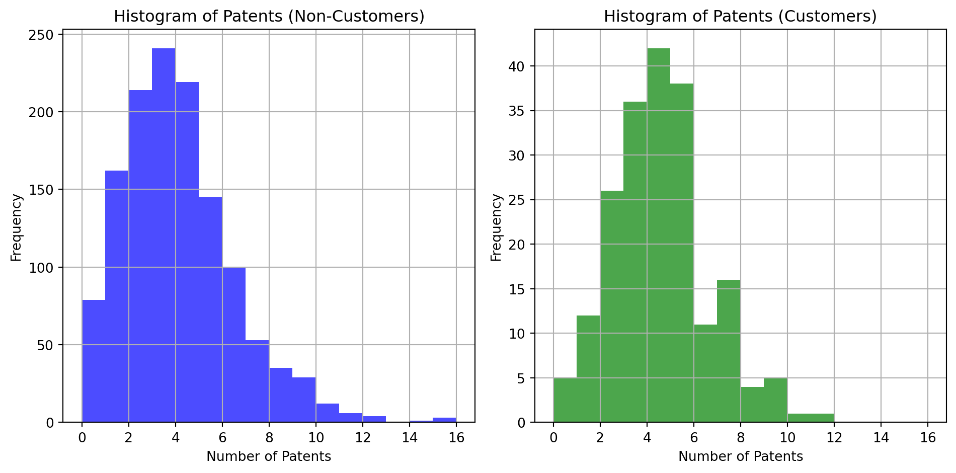
Non Customer Mean: 3.62 Customer Mean: 4.09
From the histograms and mean calculations, it appears that customers of Blueprinty tend to have a slightly higher average number of patents compared to non-customers. This could suggest a positive impact of using Blueprinty’s software on patent success, though other factors like firm age or region might also influence these results.
Comparing Regions

Region: There does not seem to be a very distinct pattern that strongly differentiates the regional distribution of customers versus non-customers, although some regions might slightly favor customer presence.
Age: Customers tend to be younger firms compared to non-customers. This might suggest that younger firms are more likely to adopt Blueprinty’s software, or it could reflect market penetration strategies targeted at newer firms.
Estimation of Simple Poisson Model
In the case of modeling the number of patents with a Poisson distribution, we start with the assumption that the number of patents awarded (\(Y\)) to each firm follows a Poisson distribution. The Poisson distribution is commonly used to model counts of events happening independently over a fixed period or in a fixed area, which fits the context of counting patents awarded over a specific time.
Poisson Probability Mass Function
For a random variable \(Y\) that follows a Poisson distribution with a rate parameter \(\lambda\) (average rate of occurrence over an interval), the probability mass function (PMF) is given by: \[ f(Y|\lambda) = \frac{e^{-\lambda} \lambda^Y}{Y!} \]
Where: - \(Y = 0, 1, 2, \dots\) is the count of patents (i.e., the number of events).
\(\lambda > 0\) is the mean number of patents awarded per firm over the interval (5 years, in this case).
\(e\) is the base of the natural logarithm.
\(Y!\) is the factorial of \(Y\).
Likelihood Function
The likelihood function for the Poisson distribution, given a sample of \(n\) observed values \(Y_1, Y_2, \dots, Y_n\), is the product of the individual probabilities for each observed value: \[ L(\lambda | Y_1, Y_2, \dots, Y_n) = \prod_{i=1}^{n} \frac{e^{-\lambda} \lambda^{Y_i}}{Y_i!} \]
This function indicates how likely it is to observe this particular set of data as a function of \(\lambda\). When we fit a model, we look for the \(\lambda\) that maximizes this likelihood, known as the Maximum Likelihood Estimate (MLE).
Log-Likelihood
For computational convenience, it is often easier to maximize the log of the likelihood because the logarithm is a monotonically increasing function. The log-likelihood of the Poisson distribution is: \[ \log L(\lambda | Y_1, Y_2, \dots, Y_n) = \sum_{i=1}^{n} \left(-\lambda + Y_i \log(\lambda) - \log(Y_i!)\right) \]
Maximizing this log-likelihood function with respect to \(\lambda\) gives us the MLE of \(\lambda\), which is particularly straightforward in the case of the Poisson distribution since the derivative of the log-likelihood function leads to a simple solution.
Using the statsmodels module we can easily implement the above, while taking into account the iscustomer status as a predictor for \(\lambda\).
| Dep. Variable: | patents | No. Observations: | 1500 |
| Model: | GLM | Df Residuals: | 1498 |
| Model Family: | Poisson | Df Model: | 1 |
| Link Function: | Log | Scale: | 1.0000 |
| Method: | IRLS | Log-Likelihood: | -3362.7 |
| Date: | Tue, 30 Apr 2024 | Deviance: | 2352.6 |
| Time: | 19:24:57 | Pearson chi2: | 2.25e+03 |
| No. Iterations: | 4 | Pseudo R-squ. (CS): | 0.006565 |
| Covariance Type: | nonrobust |
| coef | std err | z | P>|z| | [0.025 | 0.975] | |
| const | 1.2874 | 0.015 | 88.453 | 0.000 | 1.259 | 1.316 |
| iscustomer | 0.1215 | 0.038 | 3.189 | 0.001 | 0.047 | 0.196 |
Model Summary:
Log-Likelihood: The log-likelihood of the model is -3362.7, indicating the fit of the model to the data under the log link function.
Pseudo R-squared: The Pseudo R-squared value is 0.006565, which suggests that the model explains a small fraction of the variability in the number of patents.
Coefficients:
Constant (Intercept): The coefficient for the intercept is 1.2874. This can be interpreted as the log of the expected count of patents for non-customers, which exponentiated gives about \(e^{1.2874} \approx 3.62\) patents on average for non-customers.
Customer Status: The coefficient for
iscustomeris 0.1215. This coefficient is positive and statistically significant (p-value = 0.001). It suggests that being a customer is associated with a higher rate of patents. Exponentiating this coefficient gives about \(e^{0.1215} \approx 1.13\), which means customers see a 13% increase in the rate of patents relative to non-customers.
This model indicates that there is a statistically significant but relatively modest effect of using Blueprinty’s software on the number of patents received. Customers of Blueprinty, on average, receive about 13% more patents than non-customers, holding other factors constant.
Manual Implementation
The formula for the log-likelihood of the Poisson distribution is: \[ \log L(\lambda | Y) = \sum_{i=1}^{n} \left(-\lambda + Y_i \log(\lambda) - \log(Y_i!)\right) \]
In Python this looks like this:
-lambda * n + sum(Y_i * log(lambda)) - sum(log(Y_i!))
def poisson_loglikelihood(lambda_, Y):
    """
    Calculate the log-likelihood for the Poisson distribution given a lambda and an array of observed counts Y.

    Args:
    lambda_ (float): The rate parameter of the Poisson distribution.
    Y (array-like): Observed counts.

    Returns:
    float: The log-likelihood value.
    """
    return -lambda_ * len(Y) + np.sum(Y * np.log(lambda_)) - np.sum(gammaln(Y + 1))
log_likelihood = poisson_loglikelihood(lambda_, Y)
log_likelihood-3399.0629915336285A log-likelihood of -3399.06 indicates the probability of observing the given patent count data under the assumed Poisson distribution with the computed \(\lambda\). This number by itself is abstract, but it becomes meaningful when used to compare this model against others, such as models with additional variables or different distributions.
Ploting \(\lambda\)
lambda_range = np.linspace(0.5 * lambda_, 1.5 * lambda_, 400)
log_likelihood_values = [poisson_loglikelihood(l, Y) for l in lambda_range]
Using the function created we plot \(\lambda\) on the horizontal axis and the log-likelihood on the vertical axis for the range of lambdas.

Curve Shape: The plot shows a peak around the estimated \(\lambda\) (marked by the red dashed line), which is expected as this value of \(\lambda\) maximizes the log-likelihood according to our model fit. This is characteristic of the behavior of likelihood functions around their maximum values, confirming that our estimation procedure is finding a plausible maximum.
Sensitivity: The curve is relatively steep around the estimated \(\lambda\), indicating that small deviations from this value result in a noticeable decrease in log-likelihood. This suggests that the data provides a clear indication of the rate of patents, supporting the value we estimated.
The peak of the log-likelihood function tells us the most likely rate of patent awards (given the model and data), with values on either side less likely to produce the observed data.
Exploring MLE of Lambda for a Possion Distribution
To do this, we need to differentiate the log-likelihood function with respect to \(\lambda\) and set it equal to zero. The log-likelihood function, given observations \(Y_1, Y_2, \dots, Y_n\), is:
\[ \log L(\lambda | Y) = \sum_{i=1}^{n} \left(-\lambda + Y_i \log(\lambda) - \log(Y_i!)\right) \]
Taking the derivative of this function with respect to \(\lambda\), we get:
\[ \frac{d}{d\lambda} \log L(\lambda | Y) = \sum_{i=1}^{n} \left(-1 + \frac{Y_i}{\lambda}\right) \]
Setting this derivative equal to zero for maximization:
\[ - n + \sum_{i=1}^{n} \frac{Y_i}{\lambda} = 0 \]
\[ \sum_{i=1}^{n} \frac{Y_i}{\lambda} = n \]
\[ \frac{\sum_{i=1}^{n} Y_i}{\lambda} = n \]
\[ \lambda = \frac{\sum_{i=1}^{n} Y_i}{n} \]
Thus, \(\lambda_{MLE} = \bar{Y}\), where \(\bar{Y}\) is the sample mean of the observed values \(Y\). This result aligns with our intuition and theoretical understanding, as \(\lambda\) in a Poisson distribution represents both the mean and the variance of the distribution.
lambda_mle = Y.mean()
lambda_mle3.6846666666666668The Maximum Likelihood Estimate (MLE) for lambda based on the observed data is approximately 3.685. This is the average number of patents per firm over the last 5 years, which indeed serves as the MLE of lambda in our Poisson model. This result confirms our theoretical derivation and reflects the natural interpretation of lambda in the Poisson distribution as the average rate (or mean) of occurrence of the event (patents awarded).
Finding the MLE with scipy.optimize
def poisson_loglikelihood_v2(lambda_, Y):
    """
    Calculate the negative log-likelihood for the Poisson distribution given a lambda and an array of observed counts Y.

    Args:
    lambda_ (float): The rate parameter of the Poisson distribution.
    Y (array-like): Observed counts.

    Returns:
    float: The negative log-likelihood value.
    """
    if lambda_ <= 0:  # To ensure lambda is positive
        return np.inf
    return -(-lambda_ * len(Y) + np.sum(Y * np.log(lambda_)) - np.sum(gammaln(Y + 1)))
Updated version of the function above to make the absolute positive.
from scipy.optimize import minimize
result = minimize(poisson_loglikelihood_v2, initial_lambda, args=(Y,), method='L-BFGS-B', bounds=[(0.001, None)])
result
message: CONVERGENCE: REL_REDUCTION_OF_F_<=_FACTR*EPSMCH
success: True
status: 0
fun: 3367.6837722351047
x: [ 3.685e+00]
nit: 8
jac: [-2.728e-04]
nfev: 18
njev: 9
hess_inv: <1x1 LbfgsInvHessProduct with dtype=float64>Using minimize() finds the MLE of the lambda parameter for the given poisson distribution that best fits the observed data.
Estimated lambda: Approximately 3.685, which closely matches the sample mean we calculated manually and confirms our previous findings.
Optimization Status: The process converged successfully, indicating that a minimum of the negative log-likelihood function was found effectively.
Function Evaluations: It took 18 function evaluations to reach convergence, showing an efficient optimization given the simplicity of the function.
Log-Likelihood: The minimum value of the log-likelihood at the optimum lambda is about 3367.684.
Estimation of Poisson Regression Model
Next, we extend our simple Poisson model to a Poisson Regression Model such that \(Y_i = \text{Poisson}(\lambda_i)\) where \(\lambda_i = \exp(X_i'\beta)\). The interpretation is that the success rate of patent awards is not constant across all firms (\(\lambda\)) but rather is a function of firm characteristics \(X_i\). Specifically, we will use the covariates age, age squared, region, and whether the firm is a customer of Blueprinty.
def poisson_regression_loglikelihood(beta, Y, X):
    """
    Calculate the negative log-likelihood for the Poisson regression model given beta coefficients, observed counts Y, and covariate matrix X.

    Args:
    beta (array-like): The coefficient vector for the covariates.
    Y (array-like): Observed counts.
    X (2D array-like): Covariate matrix where each row corresponds to an observation and each column to a covariate.

    Returns:
    float: The negative log-likelihood value.
    """
    lambda_i = np.exp(X @ beta)
    log_likelihood = np.sum(-lambda_i + Y * np.log(lambda_i) - gammaln(Y + 1))
    return -log_likelihood
This updated function allows us to pass the covariate matrix X.
Beta Coefficients: The estimated coefficients for the model are as follows: - Intercept: beta_0 approx 1.215
Age: beta_1 approx 1.046
Age Squared: beta_2 approx -1.141
Customer Status: beta_3 approx 0.118
Region Northeast: beta_4 approx 0.099
Region Northwest: beta_5 approx -0.020
Region South: beta_6 approx 0.057
Region Southwest: beta_7 approx 0.051
Age Effects: The positive coefficient for age and the negative coefficient for age squared suggest a non-linear relationship where the number of patents increases with age to a point, after which it begins to decrease. This could represent a “peak productive period” for firms.
Customer Status: The positive coefficient for being a customer indicates that, all else equal, firms using Blueprinty’s software are expected to have a higher rate of patents.
Regional Effects: The coefficients for the regions indicate slight variations in patent rates across different regions, with some regions showing slightly higher or lower rates than the baseline (Midwest, which was dropped due to one-hot encoding).
This model provides a richer understanding of the factors influencing patent rates across firms and confirms the utility of including additional covariates to model such outcomes more accurately.
Hessian of Poisson Model with Covariats
The Hessian matrix is a fundamental component in the inference of maximum likelihood estimators. By calculating the inverse of the Hessian matrix at the optimum (MLEs of the parameters), we obtain the covariance matrix of the estimates. The diagonal elements of this matrix provide the variances (and thus standard errors) of the parameter estimates.
The Hessian also helps confirm the stability and reliability of the optimization process. A well-behaved Hessian (i.e., positive definite at the optimum) suggests that the optimization found a true maximum of the likelihood function. This is crucial for decision making and making statistical inferences.
| Coefficient | Standard Error | Standard Error (from Hessian) | |
|---|---|---|---|
| intercept | 1.215451 | 31.305234 | 0.036425 |
| age | 1.046434 | 57.308666 | 0.100487 |
| age_squared | -1.140819 | 57.254890 | 0.102494 |
| iscustomer | 0.118172 | 10.565816 | 0.038920 |
| region_Northeast | 0.098560 | 23.819037 | 0.042007 |
| region_Northwest | -0.020052 | 3.153481 | 0.053782 |
| region_South | 0.057158 | 9.626092 | 0.052675 |
| region_Southwest | 0.051278 | 13.110999 | 0.047213 |
Coefficient:
Description: This column shows the estimated values of the regression coefficients (()) for each predictor in the model. These values represent the log change in the expected count of patents for a one-unit increase in the predictor, holding other variables constant.
Interpretation:
Positive values indicate that an increase in the predictor is associated with an increase in the expected count of patents.
Negative values indicate that an increase in the predictor leads to a decrease in the expected count of patents.
For binary predictors like
iscustomer, the coefficient tells us the log change in the expected count of patents when the firm is a customer versus not a customer.
Initial Standard Error:
Description: Initially, the standard errors were calculated from an approximation of the covariance matrix obtained indirectly through the optimization process.
Interpretation: Standard errors measure the variability or uncertainty in the coefficient estimates. Larger standard errors suggest greater uncertainty about the coefficient estimate.
Standard Error (from Hessian):
Description: These standard errors are calculated directly from the Hessian matrix of the negative log-likelihood function at the estimated coefficients. The Hessian provides a second-order approximation to the curvature of the likelihood surface at the optimum.
Interpretation: Like the initial standard errors, these values measure the precision of the estimates. The smaller these values, the more confident we can be about the accuracy of the estimated coefficients.
Validating Results with Statsmodels glm()
Up to this point in the analysis, we took a “looking under the hood” approach to this case study. Using the open source statsmodels api we can easily summarize our work.
| Variable | Coefficient (Manual) | Standard Error (Manual) | Coefficient (GLM) | Standard Error (GLM) |
|---|---|---|---|---|
| Intercept | 1.215 | 0.036 | 1.215 | 0.036 |
| Age | 1.046 | 0.100 | 1.046 | 0.100 |
| Age Squared | -1.141 | 0.102 | -1.141 | 0.102 |
| Is Customer | 0.118 | 0.039 | 0.118 | 0.039 |
| Region Northeast | 0.099 | 0.042 | 0.099 | 0.042 |
| Region Northwest | -0.020 | 0.054 | -0.020 | 0.054 |
| Region South | 0.057 | 0.053 | 0.057 | 0.053 |
| Region Southwest | 0.051 | 0.047 | 0.051 | 0.047 |
Consistency: The coefficients and standard errors from the
statsmodels.GLMfunction match exactly with those computed manually using the Hessian-based approach. This indicates the correctness of our manual calculations and the model setup.Statistical Significance: The
z-valuesandP>|z|columns from thestatsmodelsoutput provide tests for the significance of each predictor. Coefficients with a lower p-value are statistically significant at common significance levels (e.g., 0.05), confirming the impact of those variables on the response variable.Age and Age Squared: Both coefficients are statistically significant with expected signs, indicating a peak effect of age on patent production.
Is Customer: The positive coefficient for this variable is statistically significant, indicating that customers of Blueprinty are likely to have higher patent counts.
Regions: Differences among regions show varying levels of significance, with the Northeast being significant, suggesting regional variations in patent counts.
Blueprinty Analysis Summary
Effect of Using Blueprinty’s Software:
The coefficient for the
iscustomervariable is positive and statistically significant. This suggests that firms using Blueprinty’s software, on average, have higher rates of patent awards compared to those that do not use the software.Quantitatively, the coefficient value (approximately 0.118) indicates that being a customer of Blueprinty is associated with an increase in the expected log count of patents. This translates into an exponential effect, suggesting that customers see about a 12.5% increase in the expected number of patents ([exp(0.118) - 1] * 100%).
Age of Firm:
- The relationship between the age of a firm and its patent success is modeled as a quadratic function, with both
ageandage_squaredbeing statistically significant. This indicates a peak effect where the number of patents increases with age up to a point, after which it starts to decline. This could reflect increasing expertise and resources over time, followed by a plateau or decline as firms age further.
Regional Variations:
- There are significant regional differences in patent success rates. For example, firms in the Northeast show a significantly higher rate of patent success compared to the baseline region (Midwest), suggesting regional disparities in innovation or business environments that could affect patent outcomes.
Conclusions:
Blueprinty’s Software: The analysis strongly supports the marketing claim that Blueprinty’s software helps increase the success rate of patent applications. Firms using Blueprinty’s software are statistically more likely to have higher patent counts, which could be attributed to the efficiency and effectiveness of the software in managing patent applications.
Policy and Strategy Implications: For Blueprinty, these findings justify strategies aimed at expanding their customer base by highlighting the positive impact of their software on patent success. Additionally, they might consider tailored marketing strategies for different regions or age groups of firms based on the differential effects observed.
Limitations and Further Research: While the results are promising, they are based on observational data, which can be prone to confounding factors not controlled in the model. Further research could involve more detailed data, potentially longitudinal studies, to better isolate the effect of the software from other factors. Additionally, exploring other variables like industry type, size of the firm, or specific features used in the software could provide deeper insights.
AirBnB Case Study
Introduction & Data Exploration
AirBnB is a popular platform for booking short-term rentals. In March 2017, students Annika Awad, Evan Lebo, and Anna Linden scraped of 40,000 Airbnb listings from New York City. The data include the following variables:
Descriptive Statistics:
Count: 40,628 listings, except for a few variables with missing values.
Dates: The dataset was last scraped on 2 dates, with the majority on April 2, 2017.
Room Type: Three types are available: Entire home/apt, Private room, Shared room (most listings are Entire home/apt).
Bathrooms: Ranges from 0 to 8, with an average of about 1.12 bathrooms per listing.
Bedrooms: Ranges from 0 to 10, with an average of about 1.15 bedrooms per listing.
Price: Ranges from $10 to $10,000 per night, with a median price of $100.
Number of Reviews: Ranges from 0 to 421, with a mean of approximately 15.9 reviews per listing.
Missing Values:
Host Since: 35 missing values.
Bathrooms: 160 missing values.
Bedrooms: 76 missing values.
Review Scores: Considerable number of missing entries in review scores (cleanliness, location, and value), with over 10,000 missing values in each category.
Handling Missing Values
Before proceeding with a regression model, it’s essential to handle the missing values, particularly in the review_scores_* and bathrooms columns, as these could be important predictors for our model. To manage these missing values we do the following:
Drop rows: where the missing values are likely to bias the results significantly.
Imputation: using mean, median, or another method depending on the distribution.
Poisson Regression
As mentioned earlier prior to any form of regression analysis, the data must be cleaned. Here we dropped the reviews columns and imputed the few missing values.
host_since: Imputed using forward fill method, as it’s a date and the forward fill helps preserve the chronological order.bathroomsandbedrooms: Missing values were filled using the median values of their respective columns, ensuring that the typical property characteristics are maintained.
The dataset is now complete with no missing values across all columns.
Poisson Regression
formula = 'number_of_reviews ~ days + room_type + bathrooms + bedrooms + price + instant_bookable'
model = glm(formula=formula, data=data_cleaned, family=sm.families.Poisson()).fit()
model.summary()| Dep. Variable: | number_of_reviews | No. Observations: | 40628 |
| Model: | GLM | Df Residuals: | 40620 |
| Model Family: | Poisson | Df Model: | 7 |
| Link Function: | Log | Scale: | 1.0000 |
| Method: | IRLS | Log-Likelihood: | -7.1526e+05 |
| Date: | Tue, 30 Apr 2024 | Deviance: | 1.3065e+06 |
| Time: | 19:24:57 | Pearson chi2: | 2.10e+06 |
| No. Iterations: | 11 | Pseudo R-squ. (CS): | 0.5694 |
| Covariance Type: | nonrobust |
| coef | std err | z | P>|z| | [0.025 | 0.975] | |
| Intercept | 2.7778 | 0.004 | 624.334 | 0.000 | 2.769 | 2.787 |
| room_type[T.Private room] | -0.1484 | 0.003 | -52.321 | 0.000 | -0.154 | -0.143 |
| room_type[T.Shared room] | -0.4054 | 0.009 | -47.041 | 0.000 | -0.422 | -0.389 |
| days | 5.012e-05 | 3.52e-07 | 142.264 | 0.000 | 4.94e-05 | 5.08e-05 |
| bathrooms | -0.1085 | 0.004 | -28.301 | 0.000 | -0.116 | -0.101 |
| bedrooms | 0.0989 | 0.002 | 49.371 | 0.000 | 0.095 | 0.103 |
| price | -0.0005 | 1.23e-05 | -38.983 | 0.000 | -0.001 | -0.000 |
| instant_bookable | 0.3744 | 0.003 | 130.444 | 0.000 | 0.369 | 0.380 |
Model Coefficients Interpretation:
Intercept: The base log-count of reviews is approximately 2.778. (or roughly two reviews per listing in this scenario)
Room Type:
Private Room: Listings that are private rooms have about 14.84% fewer reviews than entire homes/apartments, holding all else constant.
Shared Room: Listings that are shared rooms have about 40.54% fewer reviews than entire homes/apartments, holding all else constant.
Days: A unit increase in the number of days a listing has been posted increases the expected count of reviews by about 0.005%.
Bathrooms: Each additional bathroom is associated with about 10.85% fewer reviews, holding all else constant.
Bedrooms: Each additional bedroom is associated with about 9.89% more reviews, holding all else constant.
Price: Each additional dollar in price is associated with about 0.05% fewer reviews, holding all else constant.
Instant Bookable: Listings that are instant bookable are expected to have about 37.44% more reviews than those that are not, holding all else constant.